基于逻辑回归预测 NBA 新秀的职业生涯

预测 NBA 新秀的职业生涯寿命

该项目是使用 Scikit-learn 的二元分类模型来预测 NBA 新秀在提供一些信息（例如出场次数、助攻、抢断和失误等）的情况下是否会在联盟中持续服役 5 年。

---

数据集来源：数据世界

我们将重点关注：

• 1）利用热图相关性进行特征选择
• 2）逻辑回归

Part 1: 导入科学计算库并加载数据集

导入科学计算库

import pandas as pd # load and manipulate data 
import numpy as np # calculate the mean and standard deviation
import matplotlib.pyplot as plt # drawing graphs
from sklearn.model_selection import train_test_split # split  data into training and testing sets
from sklearn.linear_model import LogisticRegression # import Logistic regression from sklearn

import sklearn.metrics as metrics # import metrics 
import seaborn as sns # import seaborn for visualization 
from sklearn.preprocessing import MinMaxScaler #import min max scaler

from sklearn.metrics import confusion_matrix#confusion matrix
from yellowbrick.classifier import ROCAUC#Discriminationthreshold

import numpy as np
import pandas as pd 

import matplotlib.pyplot as plt
import seaborn as sns

加载数据集

nba = pd.read_csv('./data/nba_logreg.csv')

nba.head()

	Name	GP	MIN	PTS	FGM	FGA	FG%	3P Made	3PA	3P%	…	FTA	FT%	OREB	DREB	REB	AST	STL	BLK	TOV	TARGET_5Yrs
0	Brandon Ingram	36	27.4	7.4	2.6	7.6	34.7	0.5	2.1	25.0	…	2.3	69.9	0.7	3.4	4.1	1.9	0.4	0.4	1.3	0.0
1	Andrew Harrison	35	26.9	7.2	2.0	6.7	29.6	0.7	2.8	23.5	…	3.4	76.5	0.5	2.0	2.4	3.7	1.1	0.5	1.6	0.0
2	JaKarr Sampson	74	15.3	5.2	2.0	4.7	42.2	0.4	1.7	24.4	…	1.3	67.0	0.5	1.7	2.2	1.0	0.5	0.3	1.0	0.0
3	Malik Sealy	58	11.6	5.7	2.3	5.5	42.6	0.1	0.5	22.6	…	1.3	68.9	1.0	0.9	1.9	0.8	0.6	0.1	1.0	1.0
4	Matt Geiger	48	11.5	4.5	1.6	3.0	52.4	0.0	0.1	0.0	…	1.9	67.4	1.0	1.5	2.5	0.3	0.3	0.4	0.8	1.0

数据集中特征的描述如下所示：

Part 2: 数据探索

# check class imbalance
nba['TARGET_5Yrs'].value_counts()

1.0    826
0.0    503
Name: TARGET_5Yrs, dtype: int64

我们可以看到我们的数据有点不平衡。

# 检测空值
nba.isnull().sum()

# 删除空值
nba = nba.dropna()

nba.isnull().sum()

# 按（Target_5yrs）对所有观察结果进行分组
average_stats = nba.groupby('TARGET_5Yrs').mean(numeric_only=True)
average_stats = average_stats.T
average_stats

TARGET_5Yrs	0.0	1.0
GP	51.495030	65.826877
MIN	14.276740	19.700847
PTS	5.060636	7.891646
FGM	1.951093	3.051090
FGA	4.562425	6.718523
FG%	42.270775	45.242131
3P Made	0.232406	0.260169
3PA	0.763618	0.799031
3P%	19.378131	19.265496
FTM	0.928231	1.530872
FTA	1.324254	2.133656
FT%	69.122266	71.189588
OREB	0.713519	1.186683
DREB	1.522863	2.325061
REB	2.234592	3.511864
AST	1.230815	1.758838
STL	0.500000	0.693705
BLK	0.249901	0.436925
TOV	0.944732	1.349031

# 可视化数据
import seaborn as sns
sns.set(style="whitegrid")  # 或其他你喜欢的样式

plt.style.use('seaborn')
ax = average_stats.plot(kind='bar', stacked=True, figsize=(12, 10), alpha=0.7);
 
plt.legend(bbox_to_anchor=(1.05, 1), loc='upper left', prop={'size': 14})
plt.xlabel('Feature', fontsize=15)
plt.ylabel('Label', fontsize=15)
plt.xticks(fontsize=12)
plt.yticks(fontsize=12)
plt.title(' features values by label',fontsize=15,weight='bold');

Part 3: 基于相关性的进行特征缩减

nba.columns

Index(['Name', 'GP', 'MIN', 'PTS', 'FGM', 'FGA', 'FG%', '3P Made', '3PA',
       '3P%', 'FTM', 'FTA', 'FT%', 'OREB', 'DREB', 'REB', 'AST', 'STL', 'BLK',
       'TOV', 'TARGET_5Yrs'],
      dtype='object')

# 分离标签和特征
X = nba.drop(['Name','TARGET_5Yrs'], axis=1)
y = nba['TARGET_5Yrs']

# 绘制特性相关性图
nba.corr(numeric_only=True)['TARGET_5Yrs'].sort_values(ascending=False)

plt.figure(figsize=(15, 8))
sns.heatmap(X.corr(), annot=True, linewidths=5, fmt='.1f');

由于许多特征具有 1-1 相关性，这会产生重复的特征。 所以我们会放弃这些。

#Drop correlated features
X = X.drop(['FGA', 'FGM', '3PA', 'FTM', 'DREB'], axis=1)

X.head(1)

	GP	MIN	PTS	FG%	3P Made	3P%	FTA	FT%	OREB	REB	AST	STL	BLK	TOV
0	36	27.4	7.4	34.7	0.5	25.0	2.3	69.9	0.7	4.1	1.9	0.4	0.4	1.3

Part 4:逻辑回归分类

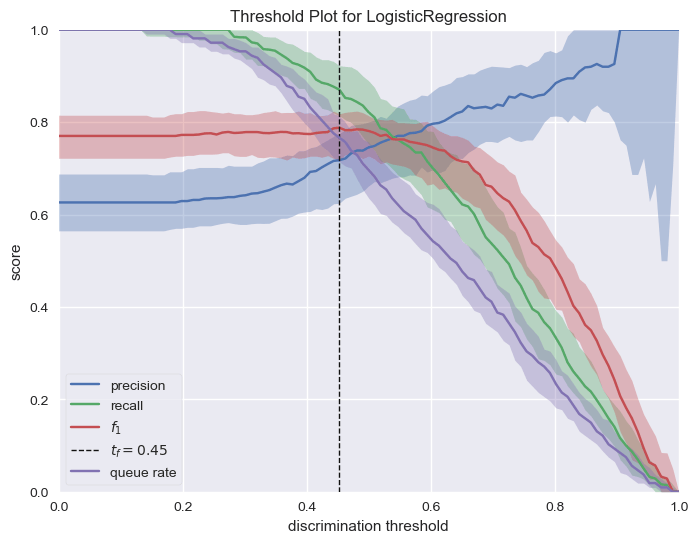
区分阈值是选择正类而不是负类的概率或分数。 通常，此值设置为 50%，但可以调整阈值以增加或降低对误报或其他应用因素的敏感度。

from sklearn.model_selection import train_test_split

#Train and Test split
X_train, X_test, y_train, y_test = train_test_split(X, y, test_size=0.2, stratify=y, random_state=42)

X_train.shape, X_test.shape

((1063, 14), (266, 14))

绘制阈值判别图

from sklearn.linear_model import LogisticRegression
from yellowbrick.classifier import DiscriminationThreshold
import warnings # import warnings
warnings.filterwarnings('ignore')
log_model = LogisticRegression()

visualizer = DiscriminationThreshold(log_model, size=(800, 600))
visualizer.fit(X_train, y_train)
visualizer.poof();

参考：https://www.scikit-yb.org/en/latest/api/classifier/threshold.html#:~:text=The%20discrimination%20threshold%20is%20the,or%20to%20other%20application%20factors 。

• 精度：精度是正确预测的正观测值的比率。精度的提高意味着误报数量的减少； 当特殊处理的成本很高时（例如，在防止欺诈或丢失重要电子邮件方面浪费时间），应该优化该指标。
• 召回率：召回率是正确预测的阳性观察结果与实际类别中所有观察结果的比率。召回率的增加会降低错过正类的可能性； 当捕获案例至关重要时，即使以更多误报为代价，也应该优化该指标。
• F1 分数：F1 分数是精确率和召回率的加权平均值。 因此，该分数同时考虑了阳性和假阴性。 直观上它不像准确度那么容易理解，但 F1 实际上比准确度更有用，特别是当你的类别分布不均匀时。优化此指标可以在精确度和召回率之间实现最佳平衡。
• 队列率：“队列”是垃圾邮件文件夹或欺诈调查台的收件箱。 该指标描述了必须审查的实例的百分比。 如果审核成本很高（例如预防欺诈），则必须根据业务要求将其最小化； 如果没有（例如垃圾邮件过滤器），可以对其进行优化以确保收件箱保持干净。

训练模型并进行预测

# 训练逻辑回归
clf = LogisticRegression()
clf.fit(X_train, y_train)

# labels prediction
threadshold = 0.35

y_pred = clf.predict_proba(X_test)
y_pred = np.where(y_pred[:, 1] > threadshold, 1, 0)

#transform y_pred array to dataframe 
y_pred = pd.DataFrame(y_pred)

y_pred

样本索引	样本预测值
0	1
1	1
2	1
3	1
4	0
…	…
261	1
262	1
263	1
264	1
265	1

266 rows × 1 columns

Part 5: 阈值判别图的调参

1) 区分度为“0.35 阈值”的混淆矩阵

from sklearn.metrics import f1_score, confusion_matrix, accuracy_score, precision_score, recall_score
#F1_Score
f1_score(y_test, y_pred)

0.7890818858560793

#Confusion matrix 
confusion_matrix(y_test, y_pred)
TN, FP, FN, TP = confusion_matrix(y_test, y_pred).ravel()
print('TN: ', TN)
print('FP: ', FP)
print('FN: ', FN)
print('TP: ', TP)

TN: 22
FP: 79
FN: 6
TP: 159

#test accuracy
accuracy_score(y_test, y_pred)

0.6804511278195489

#precision score
precision_score(y_test, y_pred)

0.6680672268907563

#recall score
recall_score(y_test, y_pred)

0.9636363636363636

2) 区分度为“0.8 阈值”的混淆矩阵

#Class label prediction
threadshold = 0.8

y_pred = clf.predict_proba(X_test)
y_pred = np.where(y_pred[:, 1] > threadshold, 1, 0)
y_pred = pd.DataFrame(y_pred)

y_pred

样本索引	样本预测值
0	0
1	1
2	0
3	1
4	0
…	…
261	0
262	0
263	1
264	1
265	0

266 rows × 1 columns

#F1_Score
f1_score(y_test, y_pred)

0.4684684684684684

#Confusion matrix
confusion_matrix(y_test, y_pred)

TN, FP, FN, TP = confusion_matrix(y_test, y_pred).ravel()

print('TN: ', TN)
print('FP: ', FP)
print('FN: ', FN)
print('TP: ', TP)

TN: 96
FP: 5
FN: 113
TP: 52

#test accuracy
accuracy_score(y_test, y_pred)

0.556390977443609

#precision score
precision_score(y_test, y_pred)

0.9122807017543859

#recall score
recall_score(y_test, y_pred)

0.3151515151515151

• 与之前的阈值配置相比，精度有所提高。 然而，准确率和召回率变得更差。

3) 区分度为“0.2 阈值”的混淆矩阵

#Class label prediction
threadshold = 0.2

y_pred = clf.predict_proba(X_test)
y_pred = np.where(y_pred[:, 1] > threadshold, 1, 0)
y_pred = pd.DataFrame(y_pred)

#F1_Score
f1_score(y_test, y_pred)

0.765661252900232

#Confusion matrix
confusion_matrix(y_test, y_pred)

TN, FP, FN, TP = confusion_matrix(y_test, y_pred).ravel()

print('TN: ', TN)
print('FP: ', FP)
print('FN: ', FN)
print('TP: ', TP)

TN: 0
FP: 101
FN: 0
TP: 165

#test accuracy
accuracy_score(y_test, y_pred)

0.6203007518796992

#precision score
precision_score(y_test, y_pred)

0.6203007518796992

#recall score
recall_score(y_test, y_pred)

1.0

• 阈值为0.2时，我们在召回率上获得了 100%。此时我们专注于召回分数。在某些情况时很有必要，例如：检测癌症。 我们不想错过任何漏报案例。

项目资源下载